Using skore with scikit-learn compatible estimators#

This example shows how to use skore with scikit-learn compatible estimators.

Any model that can be used with the scikit-learn API can be used with skore. Skore’s EstimatorReport can be used to report on any estimator that has a fit and predict method. In fact, skore only requires the predict method if the estimator has already been fitted.

Note

When computing the ROC AUC or ROC curve for a classification task, the estimator must have a predict_proba method.

In this example, we showcase a gradient boosting model (XGBoost) and a custom estimator.

Note that this example is not exhaustive; many other scikit-learn compatible models can be used with skore:

More gradient boosting libraries like LightGBM, and CatBoost,
Deep learning frameworks such as Keras and skorch (a wrapper for PyTorch).
Tabular foundation models such as TabICL and TabPFN,
etc.

Loading a binary classification dataset#

We generate a synthetic binary classification dataset with only 1,000 samples to keep the computation time reasonable:

from sklearn.datasets import make_classification

X, y = make_classification(n_samples=1_000, random_state=42)
print(f"{X.shape = }")

X.shape = (1000, 20)

We split our data:

from skore import train_test_split

split_data = train_test_split(X, y, random_state=42, as_dict=True)

╭───────────────────────────────── ShuffleTrueWarning ─────────────────────────────────╮
│ We detected that the `shuffle` parameter is set to `True` either explicitly or from  │
│ its default value. In case of time-ordered events (even if they are independent),    │
│ this will result in inflated model performance evaluation because natural drift will │
│ not be taken into account. We recommend setting the shuffle parameter to `False` in  │
│ order to ensure the evaluation process is really representative of your production   │
│ release process.                                                                     │
╰──────────────────────────────────────────────────────────────────────────────────────╯

Gradient-boosted decision trees with XGBoost#

For this binary classification task, we consider a gradient-boosted decision trees model from a library external to scikit-learn. One of the most popular is XGBoost.

from skore import EstimatorReport
from xgboost import XGBClassifier

xgb = XGBClassifier(n_estimators=50, max_depth=3, learning_rate=0.1, random_state=42)

xgb_report = EstimatorReport(xgb, pos_label=1, **split_data)
xgb_report.metrics.summarize().frame()

	XGBClassifier
Metric
Accuracy	0.896000
Precision	0.943089
Recall	0.859259
ROC AUC	0.942931
Brier score	0.086748
Fit time (s)	0.023331
Predict time (s)	0.000608

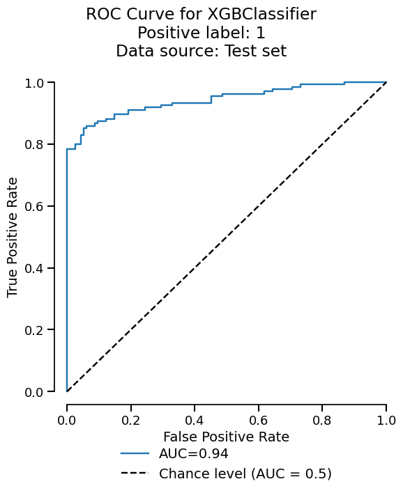
We can easily get the summary of metrics, and also a ROC curve plot for example:

xgb_report.metrics.roc().plot()

ROC Curve for XGBClassifier Positive label: 1 Data source: Test set

We can also inspect our model:

xgb_report.inspection.permutation_importance().frame()

	data_source	metric	feature	value_mean	value_std
0	test	accuracy	Feature #0	-0.0008	0.007155
1	test	accuracy	Feature #1	-0.0024	0.005367
2	test	accuracy	Feature #2	0.0016	0.003578
3	test	accuracy	Feature #3	0.0000	0.000000
4	test	accuracy	Feature #4	0.0000	0.000000
5	test	accuracy	Feature #5	0.3528	0.042275
6	test	accuracy	Feature #6	0.0032	0.003347
7	test	accuracy	Feature #7	0.0000	0.000000
8	test	accuracy	Feature #8	0.0000	0.000000
9	test	accuracy	Feature #9	-0.0024	0.002191
10	test	accuracy	Feature #10	-0.0032	0.001789
11	test	accuracy	Feature #11	0.0152	0.007694
12	test	accuracy	Feature #12	0.0024	0.006066
13	test	accuracy	Feature #13	0.0064	0.006066
14	test	accuracy	Feature #14	0.0648	0.016346
15	test	accuracy	Feature #15	0.0000	0.000000
16	test	accuracy	Feature #16	-0.0040	0.000000
17	test	accuracy	Feature #17	-0.0008	0.004382
18	test	accuracy	Feature #18	0.0064	0.007266
19	test	accuracy	Feature #19	0.0000	0.000000

Custom model#

Let us use a custom estimator inspired from the scikit-learn documentation, a nearest neighbor classifier:

import numpy as np
from sklearn.base import BaseEstimator, ClassifierMixin
from sklearn.metrics import euclidean_distances
from sklearn.utils.multiclass import unique_labels
from sklearn.utils.validation import check_is_fitted, validate_data


class CustomClassifier(ClassifierMixin, BaseEstimator):
    def __init__(self):
        pass

    def fit(self, X, y):
        X, y = validate_data(self, X, y)
        self.classes_ = unique_labels(y)
        self.X_ = X
        self.y_ = y
        return self

    def predict(self, X):
        check_is_fitted(self)
        X = validate_data(self, X, reset=False)
        closest = np.argmin(euclidean_distances(X, self.X_), axis=1)
        return self.y_[closest]

Note

The estimator above does not have a predict_proba method, therefore we cannot display its ROC curve as done previously.

We can now use this model with skore:

custom_report = EstimatorReport(CustomClassifier(), pos_label=1, **split_data)
custom_report.metrics.precision()

0.831858407079646

Conclusion#

This example demonstrates how skore can be used with scikit-learn compatible estimators. This allows practitioners to use consistent reporting and visualization tools across different estimators.